For rocket engine applications, impulse turbines are preferred, for their simplicity and light weight. Our discussion will be confined to these turbines only. Figure 6-55 shows the general arrangement of a typical single-stage tworotor velocity-compounded impulse turbine.
The following steps are essential in the design of a rocket engine impulse turbine:
The first item of importance is the selection of the proper type. A single-stage singlerotor turbine (fig. 6-8) is used if the required turbine power is low, since in this case the efficiency of the turbine has less effect on overall engine systems performance. When the avail-
able energy of the turbine working fluid and thus the gas spouting velocity C0 is relatively low, a higher turbine velocity ratio U/C0 may be achieved with a moderate turbine rotor blade speed U. As shown in figure 6-27, this suggests the use of a relatively simple single-stage single-rotor impulse turbine. We have selected this type for the A-2 stage oxidizer turbopump, at the same time taking advantage of its overall simplicity.
In most direct-drive turbopump configurations, such as the A-1 stage engine turbopump (fig. 6-63), where turbine rotating speed N and consequently turbine velocity ratio U/C0 tends to be lower than ideal, a single-stage two-rotor velocity-compounded impulse turbine (figs. 6-9 and 6-55) is selected for best results. Figure 6-27 indicates that the optimum efficiency of a velocity-compounded turbine can be achieved at a relatively low U/C0 value.
On the other hand, if a reduction gear train is provided between pumps and turbine, such as in the turbopump shown in figure 6-14, the turbine can be operated at a much higher rotating speed (over 25000 rpm ). A higher value of U/C0 can be achieved with reasonable turbine wheel size. Then a higher performance, two-stage, two-rotor, pressure-compounded impulse turbine (fig. 6-10) may be used.
2. After the type of impulse turbine has been selected, the next step is the determination of the turbine rotor size. Once the characteristics of the turbine working-fluid (i.e., inlet temperature T0, specific heat ratio γ, etc.), the turbine pressure ratio Rt, and the pump or turbine rotative speed N have been set forth, a larger diameter for the turbine rotor tends to result in a higher velocity ratio U/C0, or higher efficiency. However, it also results in higher assembly weight, larger envelope, and higher working stresses. Thus, the final selection of the turbine rotor size, and consequently the U/C0 ratio, is often a design compromise.
3. The required power output from the turbine shaft must be equal to the net input to the propellant pumps, plus the mechanical losses in the gear train (if any), plus the net power required for auxiliary drives. The required flow rate of the turbine working fluid can then be calculated by equation (6-19) after required turbine power, available energy of the working fluid (eq. 6-18), and overall turbine efficiency (estimated from
figure 6-27 for a given U/C0 ratio and turbine type), have been established.
4. Now the dimensions of the stationary nozzles, as well as those of the rotor blades, can be calculated based on the characteristics and the flow rate of the turbine working fluid.
The nozzles of most rocket engine turbines are basically similar to those of rocket thrust chambers. They are of the conventional converging-diverging De Laval type. The main function of the nozzles of an impulse-type turbine is to convert efficiently the major portion of available energy of the working fluid into kinetic energy or high gas spouting velocity. The gasflow processes in the thrust chamber nozzles are directly applicable to turbine nozzles. However, the gas flow in an actual nozzle deviates from ideal conditions because of fluid viscosity, friction, boundary layer effects, etc. In addition, the energy consumed by friction forces and flow turbulence will cause an increase in the temperature of the gases flowing through a nozzle,
above that of an isentropic process. This effect is known as reheat. As a result of the above effects, the actual gas spouting velocity at the turbine nozzle exit tends to be less than the ideal velocity calculated for isentropic expansion (from stagnation state at the nozzle inlet to the static pressure at the rotor blade inlet). Furthermore, the effective flow area of a nozzle is usually less than the actual one, because of circulatory flow and boundary layer effects. The following correlations are established for the design calculations of turbine nozzles:
Nozzle velocity coefficient kn
Actual gas spouting velocity at the nozzle exit, ft/sec
= Ideal gas velocity calculated for isentropic expansion from stagnation state at the nozzle inlet to static pressure at the rotor blade inlet, ft/sec
=C0C1(6-118)
Nozzle efficiency ηn
= Ideal gas kinetic energy (isentropic Actual gas kinetic energy at the nozzle exit
Nozzle throat area coefficient ϵnt
= Actual area Effective area of the nozzle throat (6-120)
Actual gas spouting velocity at the nozzle exit, ft/sec :
Cp= turbine gas (working fluid) specific heat at constant pressure, Btu/lb- deg F
ΔH0−1′′= isentropic enthalpy drop of the gases flowing through the nozzles, due to expansion, Btu/lb
The performance of a turbine nozzle, as expressed by its efficiency or velocity coefficient, is affected by a number of design factors, such as
(1) Exit velocity of the gas flow
(2) Properties of the turbine gases
(3) Angles and curvatures at nozzle inlet and exit
(4) Radial height and width at the throat
(5) Pitch or spacing, and number of nozzles
Design values for the efficiency and velocity coefficients of a given turbine nozzle may be determined experimentally, or estimated from past designs. Design values of nozzle efficiency ηn range from 0.80 to 0.96 . Design values of nozzle velocity coefficient kn vary from 0.89 to 0.98 . The nozzle throat area coefficient ϵnt generally will increase with nozzle radial height, with design values ranging from 0.95 to 0.99.
The cross-sectional shape (fig. 6-56) of rocket turbine nozzles is square, or, more frequently, rectangular. They are closely spaced on a circular arc extending over a part of (partial admission), or all (full admission), the circumference. Most high-power turbines use full admission for better performance.
While the gases are passing through a nozzle and expanding, the direction of flow is changing from an approximately axial direction to one forming the angle α1 (fig. 6-56) with the plane of rotation, at the nozzle exit. Thus the turning angle is 90∘−a1. The angle θΩ of the nozzle centerline at the exit usually is the result of a design compromise. Theoretically, better efficiency is obtained through the use of a smaller nozzle exit angle, since the rotor blading work is larger and the absolute flow velocity at the rotor blade exit is smaller. However, a smaller nozzle exit angle means a larger angle of flow deflection within the nozzle, which causes higher friction losses. Design values of θn range from 15∘ to 30∘. The actual effective discharge angle a1 of the gas jet leaving the nozzle tends to be greater than θn, because of the unsymmetrical nozzle shape at the exit.
A sufficiently large nozzle passage aspect ratio, hnt/bnt, is desirable for better nozzle
Figure 6-56.-Nozzles, rotor blades, and velocity diagrams of a typical single-stage impulse turbine.
efficiency. For a given nozzle height, an increase in aspect ratio can be secured by decreasing the nozzle pitch, Pn. However, a small pitch, and consequently a large number of nozzles, zn, with attendant increase in wall surface, tends to increase friction losses. The determination of nozzle pitch thus also requires a design compromise. The following correlations are established for the calculation of nozzle flow areas:
w˙t=ρ1=C1=ϵne=hnt=hne=bnt=bne=zn=θn=tn=dm= turbine gas mass flow rate, lb/sec density of the gases at nozzle exit, lb/ft3 gas spouting velocity at nozzle exit, ft/sec nozzle exit area coefficient radial height at nozzle throat, in radial height at nozzle exit, in width normal to flow at nozzle throat, in width normal to flow at nozzle exit, in number of nozzles angle between nozzle exit centerline and plane of rotation, deg thickness of nozzle partition at exit, in mean diameter of nozzles and rotor blades, in
Turbine nozzle block and inlet gas manifold assembly can be made of, for instance, welded sections of forged Hastelloy C. However, the airfoil surfaces should be blended smoothly between the defined contour and the sections.
The function of the rotor blades in an impulse turbine (figs. 6-55 and 6-56) is to transform a maximum of the kinetic energy of the gases ejected from the nozzles into useful work. Theoretically, there should be no change of gas pressure, temperature, or enthalpy in the rotor blades. In actual operation however, some gas expansion, i.e., reaction, usually occurs. Furthermore, the actual gas flow through the rotor blades deviates from ideal flow conditions because of friction, eddy currents, boundary layers, and reheating.
The velocity vector diagram shown in figure 6-56 describes graphically the flow conditions at the rotor blades of a single-stage, single-rotor turbine, based on the mean diameter dm. The gases enter the rotor blades with an absolute velocity C1, and at an angle a1 with the plane of rotation. The tangential or peripheral speed of the rotor blades at the mean diameter is U.V1 and V2, the relative velocities at the blade inlet and outlet, differ, i.e., V1>V2, due to friction losses. Ideally, the gas should leave the blades at very low absolute velocity C2 and in a direction close to axial for optimum energy conversion in the blades. The forces generated at the rotor blades are a function of the change of momentum of the flowing gases. The following correlations may be established for design calculations of the rotor blades of a single-stage, single-rotor turbine.
Tangential force acting on the blades ( lb/lb of gas flow/sec):
If there is some reaction or expansion of the gas flowing through the blades, the relative gas flow velocity at the rotor blade outlet can be calculated as
V2=kb2V12+2gJηnΔH1−2′(6-135)
Amount of reheat in the rotor blades, Btu/lb of gas flow:
qbr=(1−kb2)2gJV12+(1−ηn)ΔH1−2′(6-136)
where
a1,a2=β1,β2=C1,C2=V1,V2=Udm=ηn=ΔH1−2′= absolute gas flow angles at the inlet and outlet of the rotor blades, deg relative gas flow angles at the inlet and outlet of the rotor blades, deg absolute gas flow velocities at the inlet and outlet of the rotor blades, ft/sec relative gas flow velocity at the inlet and outlet of the rotor blades, ft/sec= peripheral speed of the rotor, ft/sec mean diameter of the rotor, in equivalent nozzle efficiency appli- cable to the expansion process in the blades isentropic enthalpy drop of the gases flowing through the rotor blades due to expansion or reaction, Btu/lb; ΔH1−2′=0 if only impulse is ex- changed
All parameters refer to the mean diameter dm, unless specified otherwise. The turbine overall efficiency ηt defined by equation (6-19) can be established for a single-stage, single-rotor impulse turbine as
ηt=ηnηbηm(6-137)
where
ηn= nozzle efficiency
ηb= rotor blade efficiency
ηm= machine efficiency indicating the mechanical, leakage, and disk-friction losses in the machine.
Equation (6-134) shows that the blade efficiency ηb improves when β2 becomes much smaller than β1. Reduction of β2 without decreasing the flow area at the blade exit can be achieved through an unsymmetrical blade design (fig. 6-56), where the radial blade height increases toward the exit. In actual designs, the amount of decrease of β2, or the increase of radial height, is limited considering incipient flow separation and centrifugal stresses. Generally, the β2 of an unsymmetrical blade will be approximately β1−(5∘ to 15∘). Equation (6-134) also indicates that ηb improves as a1 is reduced.
Design values of kb vary from 0.80 to 0.90 . Design values of ηb range from 0.7 to 0.92 .
Referring to figure 6-56, the radial height at the rotor inlet, hb, is usually slightly larger ( 5 to 10 percent) than the nozzle radial height hn. This height, together with the blade peripheral speed U, will determine the centrifugal stress in the blades. The mean diameter of the rotor blades is defined as dm=dt−hb, where dt is the rotor tip diameter. Pitch or blade spacing, Pb, is measured at the mean diameter dm. There is no critical relationship between blade pitch Pb and nozzle pitch Pn. There just should be a sufficient number of blades in the rotor to direct the gas flow. The number of blades zb to be employed is established by the blade aspect ratio, hb/Cb and the solidity Cb/Pb, where Cb is the chord length of the rotor blades. The magnitude of the blade aspect ratio ranges from 1.3 to 2.5. Design values of blade solidity vary from 1.4 to 2 . Best results will be determined by experiment. The number of rotor blades should have no common factor with the number of nozzles or of stator blades.
The blade face is concave, with radius rf. The back is convex, with a circular arc of small radius rr concentric with the face of the adjoining blade ahead. Two tangents to this arc to form the inlet and outlet blade angles θb1 and θb2 complete the blade back. The leading and trailing edges may have a small thickness tb.
The inlet blade angle θb1 should be slightly larger than the inlet relative flow angle β1. If θb1<β1, the gas stream will strike the backs of the blades at the inlet, exerting a retarding effect on the blades and causing losses. If θb1>β1, the stream will strike the concave faces of the blades and tend to increase the impulse. The outlet blade angle θb2 is generally made equal to the outlet relative flow angle β2.
The mass flow rate w˙t through the various nozzle and blade sections of a turbine is assumed constant. The required blade flow areas can be calculated by the following correlations. Note that the temperature values used in calculating the gas densities at various sections must be corrected for reheating effects from friction and turbulence.
Pb= pitch or rotor blade spacing =πdm/zb, in ρ1,ρ2 density of the gases at the inlet and outlet of the rotor blades, lb/ft3V1,V2= relative gas flow velocities at the inlet and outlet of the rotor blades, ft/sec ϵb1,ϵb2==zbhb1,hb2=bb1,bb2=θb1,θb2=tb area coefficients at inlet and outlet of the rotor blades number of blades radial height at the inlet and outlet of the rotor blades, in passage widths (normal to flow) at the inlet and outlet of the rotor blades, in rotor blade angles at inlet and out- let, deg = thickness of blade edge at inlet and outlet, in
blades and disks are shown in figures 6-53, 6-55, 6-56, and 6-57. Usually, blades are designed with a shroud, to prevent leakage over the blade tips and to reduce turbulence and thus improve efficiency. Frequently the shroud forms an integral portion of the blade, the shroud sections fitting closely together when assembled. In other designs the shroud may form a continuous ring (fig. 6−55 ) which is attached to the blades by means of tongues at the blade tip, by rivets, or is welded to the shrouds. The blades may be either welded to the disk, or attached to it using "fir-tree" or other dovetail shapes.
The main loads to which a rotor blade is exposed can be divided into three types:
Tension and bending due to centrifugal forces. -The radial component of the centrifugal forces acting on the blade body produces a centrifugal tensile stress which is a maximum at the root section. As a remedy, blades are often tapered, with the thinner section at the tip, for lower centrifugal root stresses. The centroids
of various blade sections at different radii generally do not fall on a true radial line. Thus the centrifugal forces acting upon the offset centroids will produce bending stresses which also are a maximum at the root section.
Bending due to gas loading.-The tangential driving force and the axial thrust produced by the momentum change of the gases passing over the blades may be treated as acting at the midheight of the blade to determine the amount of bending induced.
Bending due to vibration loads.-The gas flow in the blade passages is not a uniform flow as assumed in theory, but varies cyclically from minimum to maximum. The resultant loads represent a dynamic force on the blades, having a corresponding cyclic variation. If the frequency of this force should become equal to the natural frequency of the blades, deflections may result which will induce bending stresses of considerable magnitude.
Detail stress analyses for rotor blades can be rather complex. A basic approach is to counteract a major portion of the bending moments from gas loading with the bending moments induced by the centrifugal forces at nominal operating speeds. This can be accomplished by careful
Figure 6-57.-Typical rotor blade constructions.
blade design. Thus the centrifugal tensile stresses become a first consideration in blade design, while other details such as centroid location and root configuration are established later to fulfill design requirements. The following correlations are established at the blade root section where stresses are most critical.
Centrifugal tensile stress at the root section of blade of uniform cross section, psi:
Sc=0.0004572g1ρbhbdmN2(6-141)
Centrifugal tensile stress at the root section of a tapered blade, psi:
Bending moment due to gas loading at the root section, in-lb:
Mg=2zbhbw˙tFt2+Fa2(6-143)
where
ρb= density of the blade material, lb/in3hb= average blade height, in
dm= mean diameter of the rotor, in
N= turbine speed, rpm
ar= sectional area at the blade root, in 2at= sectional area at the blade tip, in 2w˙t= turbine gas flow rate, lb/seczb= number of blades
Ft= tangential force acting on the blades, lb/lb/sec (eq. (6-127))
Fa=axial thrust acting on the blades, lb/lb/ sec (eq. (6-131))
The bending stresses at the root can be calculated from the resultant bending moment. The vibration stresses can be estimated from past design data. If the blade is fitted with a separate shroud, its centrifugal force produces additional stresses at the root. The total stress at the root section is obtained by adding these stresses to those caused by the centrifugal forces acting on the blades.
The stresses in a turbine rotor disk are induced by (1) the blades, and (2) the centrifugal forces acting on the disk material itself. In addition, there will be shear stresses resulting from the torque. As seen in figure 6-55, turbine disks are generally held quite thick at the axis, but taper off to a thinner disk rim to which the blades are attached. In single-rotor applications, it is possible to design a disk so that both radial and tangential stresses are uniform at all points, shear being neglected. In multirotor applications, it is difficult to do this because of the greatly increased axial length and the resulting large gaps between rotor and stator disks.
Equation (6-144) may be used to estimate the stresses in a uniform stress turbine disk, neglecting rotor blade effects:
where
Sd=0.000114g1ρdloge(trt0)dd2N2(6-144)Sd=ρd=dd=N=t0=tr= centrifugal tensile stress of a constant stress turbine disk, psi density of the disk material, lb/in3 diameter of the disk, in turbine speed, rpm thickness of the disk at the axis, in thickness of the disk rim at dd, in
Equation (6-144a) permits estimation of the stresses in any turbine disk, neglecting effects of the rotor blades:
Sd=0.0004425g1WdriadN2(6-144a)
where
Sd=Wd=ri=ad=N= centrifugal tensile stress of the turbine disk, psi weight of the disk, lb distance of the center of gravity of the half disk from the axis, in disk cross-sectional area, in2 turbine speed, rpm
For good turbine design, it is recommended that at maximum allowable design rotating speed, the Sd calculated by equation (6-144a) should be about 0.75 to 0.8 material yield strength.
Turbine rotor blades and disks are made of high-temperature alloys of three different base
materials: iron, nickel, and cobalt, with chromium forming one of the major alloying elements. Tensile yield strength of 30000 psi minimum at a working temperature of 1800∘F is an important criterion for selection. Other required properties include low creep rate, oxidation and erosion resistance, and endurance under fluctuating loads. Haynes Stellite, Vascojet, and Inconel X are alloys frequently used. The rotor blades are fabricated either by precision casting or by precision forging methods. Rotor disks are best made of forgings for optimum strength.
Design of Single-Stage, Two-Rotor VelocityCompounded Impulse Turbines (figs. 6-9, 6-55, and 6-58)
In most impulse turbines, the number of rotors is limited to two. It is assumed that in a singlestage, two-rotor, velocity-compounded impulse turbine, expansion of the gases is completed in the nozzle, and that no further pressure change occurs during gas flow through the moving blades. As mentioned earlier, the two-rotor, velocity-compounded arrangement is best suited for low-speed turbines. In this case, the gases ejected from the first rotor blades still possess considerable kinetic energy. They are, therefore, redirected by a row of stationary blades into a second row of rotor blades, where additional work is extracted from the gases, which usually leave the second rotor blade row at a moderate velocity and in a direction close to the axial.
The velocity diagrams of a single-stage, tworotor, velocity-compounded impulse turbine are shown in figure 6-58, based on the mean rotor diameter. The peripheral speed of the rotor blades at this diameter is represented by U. The gases leave the nozzles and enter the first rotor blades with an absolute velocity C1, at an angle a1 with the plane of rotation. V1 and V2 are the relative flow velocities in ft/sec at the inlet and outlet of the first rotor blades. The gases leave the first rotor blades and enter the stationary blades at an absolute flow velocity C2, and at an angle a2. After passing over the stationary blades, the gases depart and enter the second rotor blades at an absolute flow velocity C3, and at an angle α3.V3 and V4 are the relative inlet and outlet flow velocities at the second rotor
blades. Angles β1,β2,β3, and β4 represent the flow directions of V1,V2,V3, and V4.
As with single-rotor turbines, the exit velocity from any row of blades (rotary or stationary) is less than the inlet velocity, because of friction losses. It can be assumed that the blade velocity coefficient kb has the same value for any row of blades:
kb=V1V2=C2C3=V3V4(6-145)
In a multirotor turbine, the total work transferred is the sum of that of the individual rotors:
Figure 6-58.-Velocity diagrams of a typical single-stage, two-rotor, velocity-compounded impulse turbine.
Total work transferred to the blades of a tworotor turbine, ft−lb/lb of gas flow/sec
Combined nozzle and blade efficiency of a tworotor turbine:
ηnb=JΔHE2b(6-147)
where
ΔH= overall isentropic enthalpy drop of the turbine gases, Btu/lb = total available energy content of the tur- bine gases (eq. 6−17) Equation (6−137) can be rewritten for the tur-
bine overall efficiency ηt of a two-rotor turbine as
ηt=ηnbηm(6-148)
Ideally, ηnb is a maximum for the singlestage, two-rotor, velocity-compounded impulse turbine velocity ratio
C1U=4cosa1
i.e., when U=41C1t. The workload for the second rotor of a two-rotor, velocity-compounded turbine is designed at about one-fourth of the total work.
The design procedures for the gas flow passages of the rotor and stationary blades of a single-stage, two-rotor turbine are exactly the same as those for a single-rotor turbine. However, velocities and angles of now change with each row of blades. As a result, the radial height of symmetrical blades increases with each row, roughly as shown in figure 6-55. The effects of reheating (increase of gas specific volume) in the flow passages must be taken into account when calculating the gas densities at various sections. Equation (6-136) may be used to estimate the amount of reheat at each row of blades. Also see sample calculation (6-11) and figure 6-60 for additional detail.
In the calculations for multirow unsymmetrical blades, the radial heights at the exit side of each row are determined first by equation (6-140). The radial heights at the blade inlets are then made slightly larger, approximately 8 percent, than those at the exit of the preceding row.
Design of Two-Stage, Two-Rotor PressureCompounded Impulse Turbines (figs. 6-10, 6-14 and 6-59)
An operational schematic of a typical twostage, two-rotor, pressure-compounded impulse turbine and its velocity diagrams at the mean diameter are shown in figures 6-10 and 6-59. Each stage of a pressure-compounded impulse turbine may be regarded as a single-stage impulse turbine rotating in its own individual housing. Most of the design characteristics of a single-stage turbine are applicable to the individual stages. The gas-spouting velocities C1 and C3, at flow angles a1 and a3, of the firstand second-stage nozzles, are designed to be approximately the same. V1,V2,V3, and V4 represent the relative flow velocities at inlets and outlets of the rotor blades. β1,β2,β3, and β4 are the corresponding flow angles for V1,V2, V3, and V4. The second-stage nozzles are designed to receive the gas flow discharged from the first-stage rotor blades at an absolute velocity C2, and to turn it efficiently to a desired angle a3. Simultaneously, the gases are accelerated to a desired velocity C3, through expansion to a lower pressure. The flow at the outlet of the second rotor has an absolute velocity C4 and a flow angle a4. U is the rotor peripheral speed at the mean effective diameter dm.
The total work performed in the turbine is the sum of that of the separate stages. These may be designed to divide the load equally (i.e., the
Figure 6-59.-Velocity diagrams of a typical twostage, two-rotor, pressure-compounded impulse turbine.
velocity diagrams of each stage are identical or C1=C3,C2=C4,a1=a3,a2=a4, etc.). The friction losses occurring in the first stage is passed on in the gas stream as additional enthalpy and increases the available energy for the second stage. Also, the kinetic energy of the gases leaving the first stage is largely used and not entirely lost as with a single-stage turbine. The carryover ratio Ic, i.e., the ratio of the kinetic energy actually utilized as inlet energy by the second-stage nozzles to the total kinetic energy of the gases leaving the first stage, can vary from 0.4 to close to unity. The axial distance between the first-stage rotor and the second-stage nozzle, as well as the leakages through the sealing diaphragm between stages, should be minimized for optimum carryover.
The determination of the right enthalpy drop resulting in equal work for each stage may require a trial-and-error approach, in view of the effects of reheating. Or, the proper enthalpy drop may be estimated from previous designs and test data. With the velocity coefficients for nozzles and blades given by past or concurrent experiments, equations (6-122) and (6-136) can be used to estimate the amount of reheating.
Most equations established for the singlestage turbines may be employed in the design calculations for two-stage turbines. The following additional correlations are available for the design of second stage nozzles:
$T_{2 t} \quad=$ turbine gas total (stagnation) temper-
    ature at second-stage nozzle inlet,
    ${ }^{\circ} \mathrm{R}$
$T_{2} \quad=$ turbine gas static temperature at
    second-stage nozzle inlet, ${ }^{\circ} \mathrm{R}$
$p_{2 t} \quad$ = turbine gas total pressure at second-
    stage nozzle inlet, psia
$p_{2} \quad=$ turbine gas static pressure at second-
stage nozzle inlet, psia
$C_{2}=$ absolute gas flow velocity at first-
    stage rotor blade outlet, ft/sec
$C_{3} \quad$ = gas-spouting velocity at second-stage
    nozzle exit, ft/sec
$I_{c} \quad=$ second-stage carryover ratio of kinetic
    energy
$C_{p} \quad=$ turbine gas specific heat at constant
    pressure, Btu/lb-deg F
$\gamma \quad=$ turbine gas specific heat ratio
$\Delta H_{2-3^{\prime}}=$ isentropic enthalpy drop of the gases
    flowing through the second-stage
    nozzles due to expansion, Btu/lb
$\left(A_{\mathrm{nt}}\right)_{2}=$ required total second-stage nozzle
    area, in ${ }^{2}$
$k_{n} \quad=$ nozzle velocity coefficient
$\epsilon_{\mathrm{nt}} \quad=$ nozzle throat area coefficient
From sample calculation (6-5), the following data have been obtained for the turbine of the A-1 stage engine turbopump.
Turbine gas mixture ratio, LO2/RP−1=0.408
Turbine gas specific heat at constant pressure, Cp=0.653Btu/lb−degF
Turbine gas specific heat ratio, y=1.124
Turbine gas constant, R=53.6ft/∘R
Gas total temperature at turbine inlet, T0=1860∘R
Gas total pressure at turbine inlet, p0=640 psia
Gas static pressure at turbine exhaust, pe=27 psia
Total available energy content of the turbine gases, ΔH=359Btu/lb
Turbine gas flow rate, w˙t=92lb/sec
Turbine shaft speed, N=7000rpm
Overall turbine efficiency (when using velocitycompounded wheels), ηt=58.2 percent
In addition, the following design data are set forth:
Nozzle aspect ratio =9.7
Nozzle velocity coefficient, kn=0.96
Nozzle throat area coefficient, ϵnt=0.97
Nozzle exit area coefficient, ϵne =0.95
Rotor and stator blade velocity coefficient, kb=0.89
Rotor and stator blade exit area coefficient, ϵb2=0.95
Chord length of rotor and stator blades, Cb=1.4in
Partition thickness at the exit of nozzles and blades, tn=tb=0.05in
Solidity of first rotor blades =1.82
Solidity of stator blades =1.94
Solidity of second rotor blades =1.67
(a) Determine the velocity diagrams and principal dimensions of the single-stage, two-rotor, velocity-compounded, impulse-type turbine for the A-1 stage engine turbopump, with about 6 percent reaction in rotor and stator blades downstream of the nozzles.
(b) Determine the velocity diagrams of an alternate two-stage, two-rotor, pressurecompounded, impulse-type turbine for the A-1 stage engine turbopump, with equal work in each stage and about 3 percent reaction in the rotor blades downstream of the nozzles of each stage.
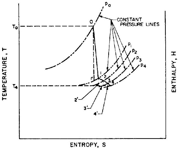
Figure 6-60.-Temperature-entropy-enthalpy diagram of the gas processes in a single-stage, two-rotor, velocity-compounded impulse turbine with small amount of reactions downstream of the nozzles.
A representative velocity diagram for this turbine is shown in figure 6-58. Figure 6-60 represents the temperature-entropy-enthalpy diagram for the gas processes involved in the operation of this turbine. The following subscripts denote the various points and processes listed:
0,1,2,3,4= Points representing inlet conditions at the nozzles; first rotor blades; stator blades; second rotor blades; and the exit conditions of the second rotor blades.
1′,2′,3′,4′= Points representing exit conditions at the nozzles; first rotor blades; stator blades; and second rotor blades, for an ideal isentropic expansion process.
0−1′,1−2′,2−3′,3−4′= Path of an ideal isentropic expansion process in the nozzles; first rotor blades; stator blades; and second rotor blades.
0−1,1−2,2−3,3−4= Path of actual processes in the nozzles; first rotor blades; stator blades; and second rotor blades.
1′−1,2′−2,3′−3,4′−4= Differences along constant pressure lines, between ideal isentropic expansion processes and actual processes, due to friction losses and reheating in the nozzles, first rotor blades, stator blades, and second rotor blades
T0= nozzle inlet total temperature = turbine inlet total temperature =1860∘Rp0= nozzle inlet total pressure = turbine inlet total pressure =640psiaΔH= overall isentropic enthalpy drop of the turbine gases = total available energy content of the turbine gases =359Btu/lbηn= nozzle efficiency =kn2=(0.96)2=0.92
Since about 6 percent of the overall isentropic enthalpy drop ΔH is assumed to occur in the rotor and stator blades, the isentropic enthalpy drop in the nozzles
ΔH0−1′=ΔH(1−0.06)=359×0.94=337.5Btu/lb
We can write:
ΔH0−1=CpT0[1−(p0p1)γγ−1]
From this, the gas static pressure at the nozzle exit
Point "2"-First Rotor Blade Exit = Stator Blade Inlet
Assume that the given 6 percent reaction downstream of the nozzles is equally divided between the two rotors and the stator. Then the isentropic enthalpy drop in the first rotor blade can be approximated as
ΔH1−2′=30.06×359=7.18Btu/lb
Using equation (6-135), the relative gas flow velocity at the exit of the first rotor blades
The gas static temperature at the exit of the first rotor blade row following an isentropic expansion
T2′=T1−ΔH1−2′/Cp=1385−7.18/0.653=1374∘R
The actual static gas temperature at the first rotor blade row exit
T2=T2′+Cpqbr2=1374+0.65341.975=1438∘R
Gas density at the first rotor blade exit
ρ2=RT2144p2=53.6×1438144×31.6=0.059lb/ft3
We use an angle β2 of 25∘ for the relative gas flow direction at the first rotor blade exits (unsymmetrical blades). The absolute flow angle α2 at the first rotor blade exits can be calculated from
Gas static temperature at the stator blade exits following an isentropic expansion
T3′=T2−ΔH2−3′/Cp=1438−7.18/0.653=1427∘R
Actual static gas temperature at the stator blade exits
T3=T3′+Cpqbs=1427+0.65318.53=1456∘R
Gas density at the stator blade exit
ρ3=RT3144p3=53.6×1456144×29.42=0.0544lb/ft3
We use an angle a3 of 35∘ for the absolute gas flow direction at the stator blade exit ( α3≅a2 ). The relative flow angle β3 at the stator blade exit can be calculated from
p4 is slightly higher than the turbine exit pressure (underexpansion), because of the reheating effects.
The gas static temperature at the second rotor blade exits following an isentropic expansion
T4′=T3−ΔH3−4′/Cp=1456−0.6537.18=1445Btu/lb
The actual gas static temperature at the second rotor blade exit
T4=T4′+Cpqbr2=1445+0.6537.73=1457∘R
Gas density at the second rotor blade exits
ρ4=RT4144p4=53.6×1457144×27.46=0.0506lb/ft3
We use an angle β4 of 44∘ for the relative gas flow direction at the second rotor blade exits (unsymmetrical blades). The absolute flow angle a4 at the second rotor blade exits can be calculated from
Assume a tapered blade with shroud, and that it is subject to approximately the same tensile stresses from centrifugal forces, as would be a uniform blade without shroud. The blades shall be made of Timken alloy, with a density ρb=0.3lb/in3. Check the centrifugal tensile stresses at the root section using equation (6-141).
From prior trial-and-error calculations, the following isentropic enthalpy drops resulting in (approximately) equal work for each stage were obtained. We assume a stage carryover ratio rc=0.91.
First-stage nozzles:
ΔH0−11=50%;ΔH=0.5×359=179.5Btu/lb
First-stage rotor blades:
ΔH1−2′=3%;ΔH=0.03×359=10.75Btu/lb
Second-stage nozzles:
ΔH2−3′=44%;ΔH=0.44×359=158Btu/lb
Second-stage rotor blades:
ΔH3−4′=3%;ΔH=0.03×359=10.75Btu/lb
Point "0"-First-Stage Nozzle Inlet
T0=1860∘Rp0=640psia
Point "1"-First-Stage Nozzle Exit=Rotor Blade Inlet
From equation (6-121), the gas-spouting velocity at the first-stage nozzle exit
C1=kn2gJΔH0−1′=0.96×223.8×179.5=2880fps
We use a value of 25∘ for the spouting-gas flow angle a1. For optimum efficiency, the peripheral speed at the rotor mean diameter
U=2cosa1C1=20.906×2880=1308fps
Using equation (6-130), the relative gas flow β1 at the first-stage rotor blade inlet can be calculated as
tanβ1=C1cosα1−UC1sinα1=2880×0.906−13082880×0.423=0.936
β1=43∘8′
The relative gas flow velocity at first-stage rotor blade inlet
V1=sinβ1C1sina1=0.6832880×0.423=1784fps
Point "2"-First-Stage Rotor Blade Exit=SecondStage Nozzle Inlet
From equation (6-135), the relative gas flow velocity at the first-stage rotor blade exit
We chose a relative exit gas flow angle β2=38∘ for the first-stage rotor blades. The absolute gas flow angle, a2, can then be calculated as
tanα2=V2cosβ2−UV2sinβ2=1736×0.788−13081736×0.616=17.25
a2=86∘40′
The absolute gas flow velocity at the firststage rotor blade exits
Since C3=C1, the remainder of the secondstage velocity diagram is the same as that of the first stage, i.e., a3=a1=25∘;β3=β1=43∘8′; V3=V1=1784fps;a4=a2=86∘40′;β4=β2=38∘; C4=C2=1070fps;V4=V2=1736fps.
From equation (6-129), the turbine rotor mean diameter
dm=πN720U=π×7000720×1308=42.7in
From equation (6-147), the combined nozzle and blade efficiency
Comment: The overall efficiency of the pressure compounded turbine is higher than that of design (a). However, a relatively large dm is required (weight, size).
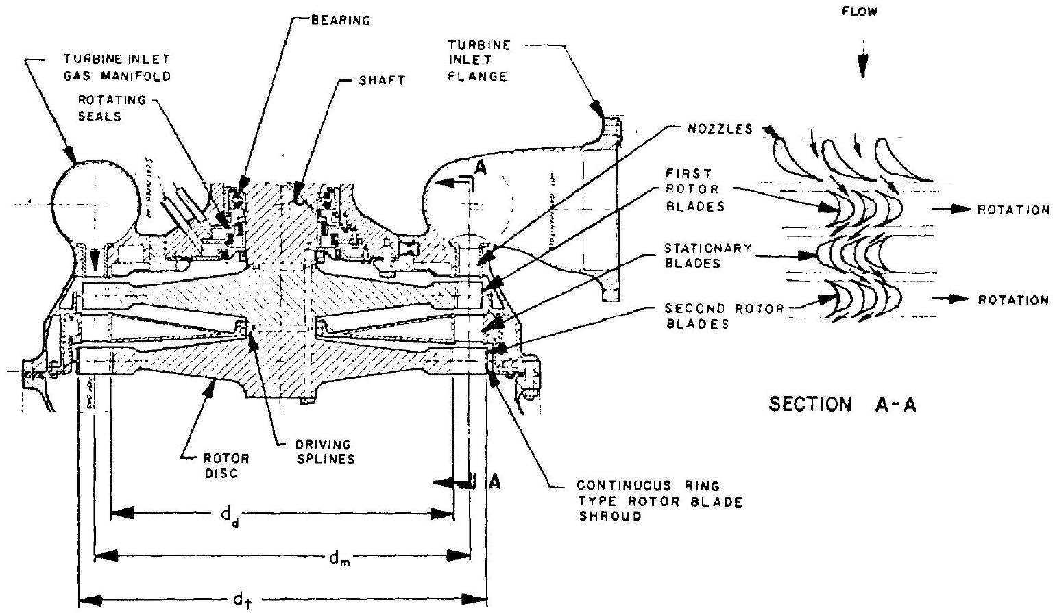 Figure 6-55.-Typical single-stage, two-rotor velocity compounded impulse turbine.
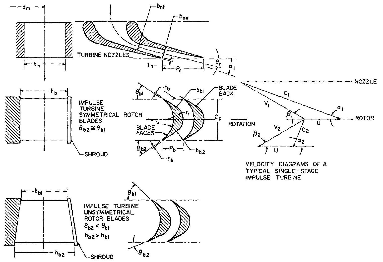 Figure 6-56.-Nozzles, rotor blades, and velocity diagrams of a typical single-stage impulse turbine.
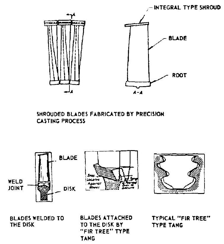 Figure 6-57.-Typical rotor blade constructions.
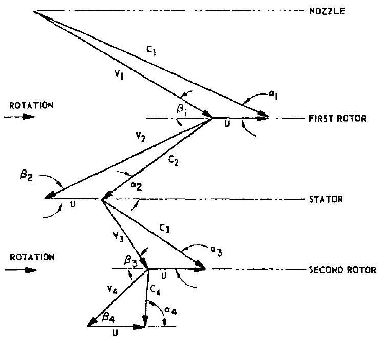 Figure 6-58.-Velocity diagrams of a typical single-stage, two-rotor, velocity-compounded impulse turbine.
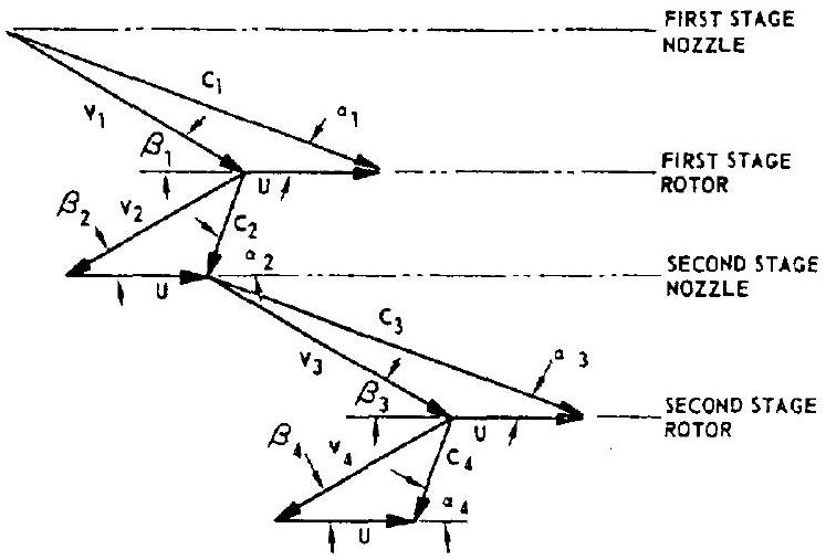 Figure 6-59.-Velocity diagrams of a typical twostage, two-rotor, pressure-compounded impulse turbine.